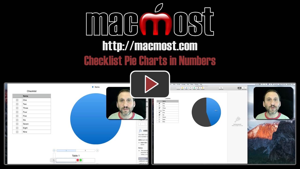
Learn how to create a Numbers spreadsheet with a checklist and pie chart that tracks your progress through the checklist. To do this, you'll need the functions COUNTIF and COUNTA.
▶ You can also watch this video at YouTube.
▶
▶ Watch more videos about related subjects: Numbers (210 videos).
▶
▶ Watch more videos about related subjects: Numbers (210 videos).


I found this to be very useful. Thank you Gary.
Is there a method that could be applied whereby the colour of the pie segment could change according to the percentage value. For example, red if = 66% ?
Eric: Nice idea, but I don't think it is possible, sorry. I suppose if you wanted to put a lot of work into it, you could create another table or set of cells to get it done. For instance, if A1 was false and B1 was true, then A2 could map to A1, B2 could use an IF function to contain B1 if less than 66% and 0 otherwise, and C2 could use an IF function to contain 0 if less then 66% and B1 otherwise. Then pie chart A2, B2, C2 instead of A1 and B1. The color for C2 would be red.