11/9/11
11:05 am

MacMost Now 629: iWork Numbers Cell Formatting

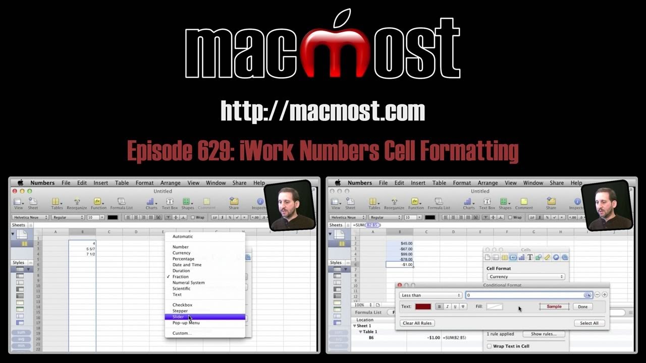
There are many options for formatting cells in iWork Numbers. You can choose the number of decimal places, or use fractions. You can format as currency or choose a different base system. You can choose from a variety of date and time formats. You can also create steppers, sliders and pop-up menus to make it easy to change values to cells. Conditional formatting allows you to have cells that change color and style with certain values or ranges.

You can also watch this video at YouTube (but with ads).

Video Transcript: Hi, this is Gary with MacMost Now. In today's episode, let's look at formatting cells in iWork Numbers. So, here I am in Numbers, and I've got a cell here with a number in it. Now I want to add some formatting to it. One of the most basic examples is making forced decimal places. So, for instance, instead of seeing 4, see 4.0. If the next number is 5.7, you can see how I've got two different formats here; it'd be nice to have them be about the same. So, I can do that in the toolbar here. If you don't see the formatting toolbar, you can go to view and hide and show format bar. Now, if I have that cell selected, I can use these buttons here to simply add more decimal places that are automatically there even if they're zeros, or take them away. And you can see I can even do that here on this cell below, I can take it away, and it'll round it from 5.7 to 6. If I want to have it be uniform for the entire column, I can select the column, and I can use those buttons there. Now, I also have some easier format buttons right there; for instance, if I wanted to format these numbers as currency, I click on the dollar sign there, and it does that. Um, I can then go and do it as a percentage if I want. I also have a pull-down menu with a bunch of different options here. For instance, I can even do fractions. I can slide fractions and say, uh, go up to just one digit of fractions, and you can see it actually puts 5 5/7 there and I can add a new number now that's been formatted like that. So let's say if I do 7.5, I can see it formats it, shows it as 7 1/2. Now, in addition to using this little pull-down menu here, I can also go to view, show inspector, and that'll bring up the inspector here, and I can look at cell format, and I get the same options here, sometimes* it's just easier to use it in Inspector. So, I can change to different things here. For instance, I can go to Duration and have it set for hours. So, uh, the 7.5 becomes 7 hours and 30 minutes. I can slide this along here and actually change that if that was supposed to be, uh, if I wanted that to be formatted in minutes, seconds, or days, or even weeks. I have a lot of different options there. You can pull down - change the format completely to something like that. One interesting one here is I can change numerical systems, so I can actually go, say, to another base, like, for instance, I can go to base 16, press the decimal. If I enter in a number like 42, I can see that changes to 2A. There. And I can go down and change to base 2 for binary. Under currency, here, I've got a lot more options. I can choose the symbol, the number of decimal places, uh, choose to have it conditionally changed to red if it's a negative number. So, for instance, if I enter in here, -9, see it does it like that, and I've got the ability to add thousands separators as well, uh, do it in accounting style with the dollar sign all the way over there on the left. You can also set formatting for dates, uh, so I have a list of dates here - go to date and time, and I can choose from one of these many different date formats here, depending upon what I want. One cool thing you can do is you can choose a cell, and you can set the format to a stepper, or a slider. So, a stepper, I can give a minimum, maximum, and increment. And a way to display it as a general format there, and when I'm done, if I go over to this one here, instead of - see, I can just edit the number here, here I don't edit, I actually would go up or down using these arrow keys. Likewise, if I change it to a slider, I get the same controls here, but if I wanted to actually change the value, I can actually slide it up and down. That slider only appears when I've selected that number. It's very useful if you're making spreadsheets, uh, so you can do computations and you want to be able to play with some of the numbers. Another thing you can do is select a cell and set several values to appear in a popup menu. So, for instance, here's just, uh, 1, 2, 3, let's change that to, uh, 10, 20, 30, so, perhaps there are several different ways you can represent a number. You can add more, so we'll add 40, and then when I've selected this cell here, I can actually choose one of these values. Now, let's take a look at something called conditional formatting. An example, we've got four numbers here and the total there, the sum of these four numbers. Suppose maybe this is receivables, payables, and I want to get kind of an alert there, we can put this being red and in bold when it's a negative number and being in green when it's a positive number. So, let me select it, and under cell format I can click conditional format, show rules, and it brings up this dialogue right here. Now, I can choose a rule, and what I'm going to choose in this case is if it's less than 0, then I'm going to edit the rule here,set the text to red, bold, and done, and I can see it's a negative number there. So what happens if I were to change a number like this 99 to 101, and now it's a positive number; you can see that it isn't red. Now, I can add an additional rule here - select that cell, add another one, and say if it's greater than or equal to 0, then it's not going to be bold, it's just going to be a green color. So now when I change the number here, make it a positive result, you can see conditional formatting changes that cell automatically. You can also use conditional formatting on a variety of other things, like for instance in this column how I listed dates, I can choose a rule that if the date is in the, say, last 7 days, then change the text to purple, and done. You can see that those last two days which are in the last seven days are purple, and you can change it to be if it's in the next seven days, do the same thing. So, I end up basically with the dates being highlighted depending on how close they are to today's date. Now, if I close this spreadsheet and open it up again a week later, you'll* actually show me different dates highlighted here, so I can kind of create a chart that always highlights the dates that are closer to the ones that are today.

Comments: 33 Responses to “MacMost Now 629: iWork Numbers Cell Formatting”

Terry Riegel

13 years ago

I am trying to use conditional formatting based on a checkbox found in another cell. Any Idea how to do this?

Gary Rosenzweig

13 years ago

I don't think you can. It only works with the data in that cell.

George Davies

13 years ago

Do you have a custom format to store valid email addresses?

Jeff

12 years ago

=if(k7="","",K7/L7*60) where K7 =distance and L7= speed this formula returns a time format minutes and tenths of minutes. I need it to return the result in hours, minutes, seconds then the column that returns this result needs to be added up with other time results and come up with a total in hours, minutes,seconds. As in excel is there a way to create a macro to clear all user inputs so the spreadsheet can be re-used with all formulas remaining

Char

12 years ago

New to Mac. I've always used Excel. Trying to format a cell in Numbers to enter blood pressure readings: i.e.: in a format that lets me enter as follows: 120/70
I see the format selections. But so far none have let me use the above format.
Help!

Gary Rosenzweig

12 years ago

What was the name of the format you used in Excel to do this?

Rick King

12 years ago

How do I get the Pop-up Menu cell format to propagate to a new row below without having to format the cell each time I add a row? Trying to format the whole column doesn't work.

Gary Rosenzweig

12 years ago

Not sure how you are trying to do this, but it works for me. I created a column with 5 rows, each with the same pop-up menu. I removed all other rows, so there are no blank rows at all, and inserted a footer row. So I had header row, 5 rows with the same pop-up menu, and a footer row. I then dragged the tab at the bottom left corner of the table and extended the table to add 10 more rows. Each of the new rows had a perfect copy of the pop-up menu.

Marinka

12 years ago

Hi Gary,
I had the same problem as Rick, but I think that the problem lies in categorizing.
It works fine on a straight-forward table, but as soon as you start categorizing the cell-format doesn't copy when adding a row.
Do you know if there is a solution to that?
Thanks,
Marinka

Gary Rosenzweig

12 years ago

No, sorry. I rarely use categorizing so I haven't run into it.

alan airdrie

12 years ago

how do i do the small "0" when i am typing degrees centigrade

Gary Rosenzweig

12 years ago

Normally, when working in a text or word processing document, you use Shift+Option+8 to get the degrees symbol. But you don't want to do that when using numbers in cells in Numbers -- it will think of the content of the cell as a text string, not as a number. So leave out the degrees symbol.

Jack

12 years ago

In need to work a rule so that if one column has a time and the next column has another time so that the difference of this can be reflected as text e.g
8:00, 13:00 difference = 5 so this is > 4 = Not acceptable? or <4 is Acceptable

Gary Rosenzweig

12 years ago

Look into using the IF function or one of the others like it.

Dustin

12 years ago

I have a pop-up menu in Numbers, I would like to allow the user to enter custom data if needed, is this possible? If not is there another way to do something similar to a list that will allow custom data?

Gary Rosenzweig

12 years ago

They could just delete the pop-up and enter their own data. Select, delete, type.

Dustin

12 years ago

AWESOME! Thank you!

rod

12 years ago

Hi Gary,

Does Numbers offer a way to have a pop up calendar for a cell? When you click a cell, a calendar appears and then you can click on the date and that date would appear in the cell?

Thanks for your input.

Gary Rosenzweig

12 years ago

No, sorry, I don't think that is an option.

JBC

12 years ago

Use custom format. You can add/subtract any symbol, number, etc. Use dropdown menu for each element.

Steve

12 years ago

How do I formatt cells to add and subtract time

Hours and mins on the 24 hour clock
Many thanks
Steve

Gary Rosenzweig

12 years ago

http://macmost.com/using-time-and-duration-values-in-numbers.html

Sara McGinnes

12 years ago

Hi Gary, Here's a baby question: I can format a date column to forward one day for the next row, after row by selecting the date and pulling it to the next row. I haven't been able to automatically enter each row one week ahead. Is this possible in Numbers 8. If so, can you tell me how?
Thanks a lot,
Sara

Gary Rosenzweig

12 years ago

So you want to fill in cells with a series of dates? I cover that here: http://macmost.com/filling-cells-in-numbers.html

Drew

12 years ago

Thanks new user - helped me out. :)

DAVID

12 years ago

Hello Gary, i bought your book My Pages and i really like it so easy to follow, i was wondering if you have a book tutorial for Numbers too! Thanks!

Gary Rosenzweig

12 years ago

Thanks! No, just Pages. I've got lots of Numbers tutorials here at MacMost, tho.

Susan

12 years ago

Is there a way to format a series of 10 numbers in a cell to look like a telephone number (111) 111-1111?

Gary Rosenzweig

12 years ago

Sure. Use the Custom format. Then play around with the interface there to create one like: (###) ###-####. But the # symbols need to be taken from the bottom portion of the interface. So you'll need to experiment.

12 years ago

how to write a code that if one cell number is more than another cell number make the text green, else make the text red
=If(B4>B4, text=green,text=red)
thanks

Gary Rosenzweig

12 years ago

You don't use a formula for that. You use conditional formatting. Watch the video.

Sheila

12 years ago

How do I format the cells to be text? I need some of my cells to be an equal sign and a number, but of course numbers thinks that I am inputting a formula, which I am not. This is driving me crazt. There does not seem to be a text format, or at least i can;t find it.

Gary Rosenzweig

12 years ago

Select the cell. Then from the format bar, choose the Text format. (look where it has 1.0, $, %, checkmark, then a menu button -- click on the menu button and choose Text).
Then immediately type =whatever.

Comments Closed.

MacMost Now 629: iWork Numbers Cell Formatting

Comments: 33 Responses to “MacMost Now 629: iWork Numbers Cell Formatting”

Welcome to MacMost

Free Weekly Newsletter

MacMost Online Courses

Keyboard Shortcuts PDF

Connect with MacMost

MacMost Sections

Popular Tutorials

Information